

Accelerometers: What do I use?

In Part 1, we examined how accelerometers are made, the types of materials used as piezoelectric elements, the role of external charge amplifiers versus integral designs, 3-wire versus IEPE1 2-wire devices, and compression-mode versus shear-mode designs. In Part 2 of this series, we turn our attention to high-level selection criteria in deciding whether to use a sensor with a native acceleration output versus a velocity output and, if velocity, whether to use a piezo-velocity sensor or a moving coil design.
1 Integrated Electronic Piezoelectric
Acceleration, velocity, and displacement – back to basics
At first glance, knowing that we can mathematically covert between acceleration, velocity, and displacement, one might be tempted to conclude that there is no need for any sensor other than acceleration – the other measurements can be derived. And indeed, we can mathematically derive each from the others using rates of change. In fact, Newton described each of these in his laws of motion as rates of change of one another using his newly-invented calculus2 to describe the relationships:
However, while these relationships are mathematically true, the realities of signal integration and differentiation with electronic circuits limit their application in the real world of industrial sensors. In particular, a mathematical differentiation circuit (so-called “ideal integrator”) introduces too many problems to reliably produce a velocity signal from a displacement3 signal. Instead, integrator circuits are used to produce velocity from acceleration and displacement from velocity. While still imperfect, these circuits are far better than differentiator circuits – particularly when only a single integration stage is used (i.e., acceleration to velocity or velocity to displacement) versus double integration (i.e., acceleration to displacement).
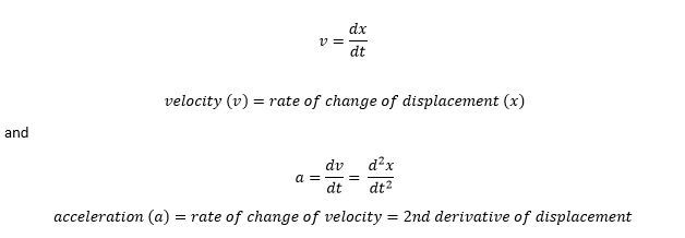
There is an even more fundamental problem, however, with simply integrating acceleration signals to arrive at displacement signals and that is the difference between absolute and relative measurements. Absolute measurements are made relative to free space – not some other part of the machine casing or structure that is vibrating. The measurements we make with casing-mounted accelerometers or velocity sensors are thus absolute measurements: the vibration relative to free space. In contrast, the measurements we make with proximity probes are always relative measurements: one part of the machine’s motion relative to another. For radial vibration, it is generally the vibrating/rotating shaft relative to the vibrating casing. For thrust position, it is generally the thrust collar (or shaft end) relative to the casing. With a proximity probe observing shaft vibration, the displacement we measure is the relative motion between the shaft and the mounting surface (usually the bearing housing) – not the motion of the bearing housing relative to free space as we would measure with a seismic sensor. Figure 1 below illustrates this issue:
Thus, if we integrate the output of the velocity sensor (or double-integrate the output of the accelerometer) in Figure 1, we will indeed get a displacement reading – but this is not shaft displacement, it is housing displacement relative to free space.
The next logical question is why we are interested in relative motion instead of absolute motion, and thus why the emphasis on proximity probes in machines with fluid-film bearings. The answer is quite simple: it is the relative motion between the moving and stationary parts of the machine that are of interest because there is a finite amount of clearance between rotors and bearings, seals, casings, etc. When these clearances are exceeded, the machine is damaged, entrained gases or liquids (often flammable and/or toxic) escape, and ensuing undesirable consequences occur. The absolute motion of the shaft is not of interest in these situations but rather the relative motion between the shaft and these stationary parts.
2 The simple question, “who invented calculus?” is perhaps the largest controversy ever to touch the field of mathematics. Historians have concluded, however, that Newton (England) and Leibniz (Germany) invented calculus quite independently of one another within the decade between 1665 and 1675, even though neither one immediately published his results. Regardless, both correctly bear the prestigious title “Inventor of Calculus.”
3 A very early version of the Bently Nevada Seismoprobe® sensor actually used – as the name implies – a proximity probe to produce a seismic velocity measurement by differentiating the displacement signal. However, it suffered from numerous problems, was quickly abandoned, and true moving-coil sensors were developed that were far more reliable and gave a native velocity output. The trademark, however, stuck and can still be found on many of Bently Nevada’s moving-coil devices to this day, helping distinguish them from piezo-velocity sensors which carry the Velomitor® trademark.
Signal strength
Another important consideration when selecting a transducer (and another reason why we do not use an accelerometer for everything and simply integrate in software or firmware) is the strength of the signal based on the native output of the sensor.
To understand this, we will contrast the output from two sensors with identical sensitivities per engineering unit. For the accelerometer, it will be 100mV/g. For the velocity sensor, it will be 100mV/in/sec. Both are typical of commercially available industrial sensors used in practice.
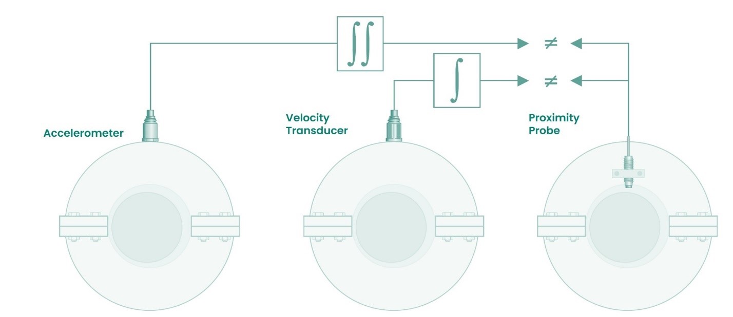
Let’s consider the 1X (running speed) amplitude of the ensuing signal from each sensor on a machine running at 600 rpm (10 Hz). We will further assume a rough-running machine with a velocity reading of 8 mm/s (0.32 in/s) of casing vibration. Using a vibration calculator or nomograph (Figure 2) that converts between sinusoidal acceleration, velocity, and displacement for a single frequency, this corresponds to 0.5 m/s2 (0.051 g’s) acceleration. In other words, our velocity sensor will give an output of 32mV while our acceleration sensor will give an output of only 5.1 mV. The velocity sensor’s output is thus more than six times stronger, resulting in a much better signal-to-noise ratio.
In general, the lower we go in frequency or machine speed, the lower our acceleration amplitudes will be relative to velocity. Indeed, when we consult a typical vibration nomograph such as Figure 2, the velocity is often given as horizontal lines because it tends to be less impacted by shaft rotative speed than either displacement or acceleration. For a given velocity level, the displacement amplitudes increase as we decrease in frequency; the acceleration levels decrease. As we increase the frequency, the converse is true: the acceleration amplitudes increase and the displacement levels decrease. This is precisely why an acceleration amplitude of 0.5 g’s pk on a machine running at 10,000 rpm is not cause for concern (0.18 in/sec pk) but a cause of tremendous concern on a machine running at 100 rpm (18.4 in/sec pk)!
When selecting a seismic sensor for casing vibration, look at the range of frequencies you wish to monitor and choose a sensor with a native output that will give the best signal strength. For example, if you are protecting a machine based on casing velocity, it is usually advisable to use a sensor with a native velocity output rather than to integrate an acceleration signal. This is particularly true for machines running at speeds below 3600 rpm.
Moving-coil velocity sensors
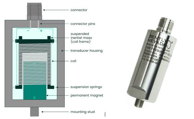
For many years, the only types of velocity sensors available for machinery monitoring were those using a moving-coil design. The concept is simple and involves little more than a coil of wire and a permanent magnet. As the magnetic field and the coil move relative to one another, a voltage is induced in the coil and is directly proportional to the velocity of this motion. Indeed, this is exactly the same principle used in a generator where a rotating magnetic field (rotor) induces voltage in a stationary coil (stator). In the case of a velocity sensor, however, we have linear back-and-forth motion rather than rotative motion. Because there must be relative motion between the two parts, the sensor is constructed such that either the magnet moves while the coil remains stationary, or vice-versa. In practice, it is generally easiest to construct a moving-coil sensor such that the magnet moves with the case of the sensor while the coil (suspended on spring supports) remains relatively motionless. Ironically, one can thus think of the sensors as a moving-magnet (rather than moving-coil) design in that sense. Figure 3 shows a cutaway drawing of such a sensor.
4 This nomograph presents displacement as a pk value rather than pp. To convert to pp, multiply by 2.
As can be imagined, if the sensor of figure 3 is turned on its side to measure horizontal rather than vertical vibration, the coil suspension will behave differently than if oriented vertically. Moving-coil devices are generally designed differently for vertical mounting versus horizontal mounting (or other mounting angles relative to vertical) and for this reason the mounting orientation must be known at time of ordering unless the design is such that it can accommodate any mounting angle.
Moving-coil sensors are usually 2-pin devices and the polarity is simply reversed if the leads are reversed. This phase reversal is usually not a problem unless you are balancing a machine, in which case you will want to know whether a positive-going signal reflects motion away from the mounting surface or towards the mounting surface. Even then, the absolute polarity is not as important as simply remaining consistent with the connections so that the phase is always consistent as well. The two pins are generally denoted “A” and “B”. Bently Nevada velocity sensors, whether moving-coil or piezoelectric in design, adhere to the convention that motion Pin A becomes positive with respect to Pin B when the applied velocity is from the base to the top of the transducer.
Some older moving-coil devices provided by Bently Nevada used 3 pins and allowed a bias voltage to be applied. The velocity signal then rode on top of this bias, much as a proximity probe AC component rides on top of its DC bias (gap voltage). This was done to allow more robust OK checks. With the advent of velocity sensors using piezoelectric designs (such as the Bently Nevada Velomitor® sensor), the use of moving-coil devices has diminished considerably. Among other advantages, so-called “piezo-velocity” sensors use a bias current that permits robust OK checks.
Piezo-velocity sensors
In Part 1 of this article series, we discussed piezoelectric accelerometers. A piezo-velocity sensor is nothing more than an accelerometer with embedded circuitry that not only converts charge to voltage, but also provides signal integration and thus gives a velocity output instead of an acceleration output. Some piezoelectric velocity sensors, such as the Bently Nevada 3309005, provide both a velocity output and an acceleration output. However, most such sensors provide only a velocity output, such as the Bently Nevada Velomitor® family including the 330500, 330525, 330750, 350752, and 190501.
By embedding the integration stage into the sensor, noise and other issues are minimized and allow the sensor to behave for all intents and purposes as a velocity sensor with a native velocity output – not an accelerometer.
Piezo-velocity sensors began to appear in the market in the mid- to late-1980s and quickly displaced moving-coil sensors for a variety of reasons:
- They had no moving parts to wear out
- They could be mounted at any orientation
- They had a superior ability to tolerate transverse (cross-axis) vibration without wearing out or influencing the signal in the primary axis
- The could provide a dual output (both acceleration and velocity) if desired using embedded electronics
The Bently Nevada 330500 was the first sensor in the Velomitor® family to be released. It was followed by several other variants including the Velomitor® XA (eXtended Applications – a ruggedized version of the basic 330500), the Velomitor® CT (Cooling Tower applications), and a high-temperature version for gas turbines and other machines incurring very high temperatures at the transducer mounting surface.
5 The 330900 High-Temperature Velocity and Acceleration Sensor (HTVAS) uses an external charge amplifier / integrator / signal conditioner due to the very high surface mounting temperature intended for the sensing element.
Is there still a place for moving-coil sensors?
With the many advantages of piezo-velocity designs, this is a natural and important question. The short answer is “yes – there is still a viable place for moving-coil designs”. Moving coil designs do not require external power as they are so-called “self-generating” sensors. Gas turbine manufacturers such as General Electric created turbine control systems with integrated vibration monitoring that assumed the use of moving-coil velocity sensors. As such, they were incapable of providing sensor power to the velocity transducers and made retrofitting with newer piezo-velocity designs more difficult. Bently Nevada can assist in upgrading to newer sensors with superior performance and no moving parts to wear out, but the incumbent casing vibration sensors on industrial gas turbines will generally be of moving-coil design.
Another place where moving-coil devices excel is in extremely low-frequency applications. Consider the Bently Nevada 330505 low-frequency velocity sensor shown in Figure 3. Using the nomograph of Figure 2, and assuming that we are measuring vibration at a typical hydroelectric turbine running speed of 90 rpm (1.5 Hz), we can see that with 10 mm/s of casing velocity (a relatively normal amount of vibration), this corresponds to only 0.00942 m/s2 (0.00096 g’s) of acceleration. While the 330500 provides an output of 200 mV at this vibration level, a typical accelerometer with a 100 mV/g sensitivity would provide a signal of only 96 microvolts (not millivolts)! This is well beneath the noise floor of most accelerometers, precluding their suitability for such applications.
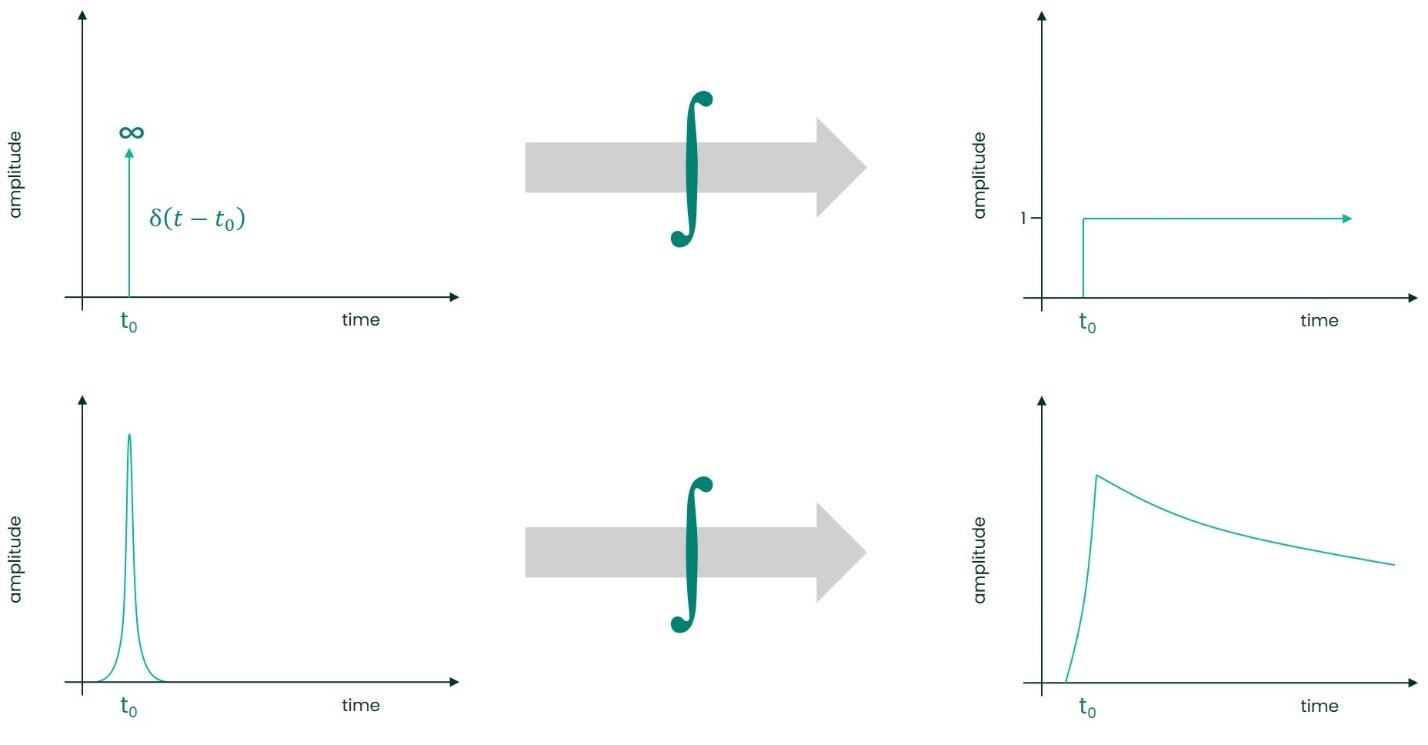
Impulse signals
Integrated accelerometer signals can be problematic when impulsive forces are present. To understand why issues can occur, consider what happens mathematically when we integrate an ideal impulse6 function: we get a step function as shown in Figure 4.
In real mechanical systems, we cannot physically have an ideal impulse function, but the idealized mathematical model helps us understand what an integrator circuit will do when something approaching an impulse is processed: it results in a rapid rise to a large value followed by a slow decay to zero.
Now, consider how a monitoring system handles a signal such as the step-like function in the lower-right of Figure 4: it sees a large DC value that exceeds the OK limits and will thus treat it as a NOT OK condition.
When piezo-velocity sensors first appeared on the market they performed very well on most machines with a notable exception: reciprocating compressors subject to impulsive forces. The phenomenon described above (integration of an impulsive signal) would cause the monitoring system to go “NOT OK” in the presence of these impulses. The sensor was not actually defective and the machine was not actually in mechanical distress. The sensor was merely responding exactly the way an integrator handles an impulsive signal. It is one of the ways in which a native velocity sensor differs from a native acceleration sensor that is integrated. Regardless, the benefits of piezo-velocity sensors still vastly outweigh the drawbacks and rather than reverting to moving-coil sensors for reciprocating compressors, Bently Nevada developed special ways of handling circuit OK checks from piezo-velocity sensors on these machines. As a result, Bently Nevada introduced recip-specific recommendations and configuration options for OK checks beginning with our 3500/70M reciprocating compressor impulse/velocity monitor. Subsequent systems such as Orbit 60 incorporate these as well.
Although most machines outside of reciprocating compressors are not subject to impulse/impact forces in normal operation, it is useful to remember that piezo-velocity sensors are – at their core – an integrating accelerometer, not a native velocity sensor, and will thus respond as shown in Figure 4 to impulse/impact excitation. Indeed, this can be easily ascertained by tapping a piezo-velocity sensor with a screwdriver and observing its time domain response on a voltmeter or oscilloscope.
6 The so-called “unit impulse function” or “Dirac delta function” is an idealized function with infinitesimal duration and infinite amplitude. The closest thing in nature to such an occurrence is probably a lightning bolt. Real impulsive forces in machinery vibration occur as mechanical impacts of very high amplitude and very short duration.
Application examples
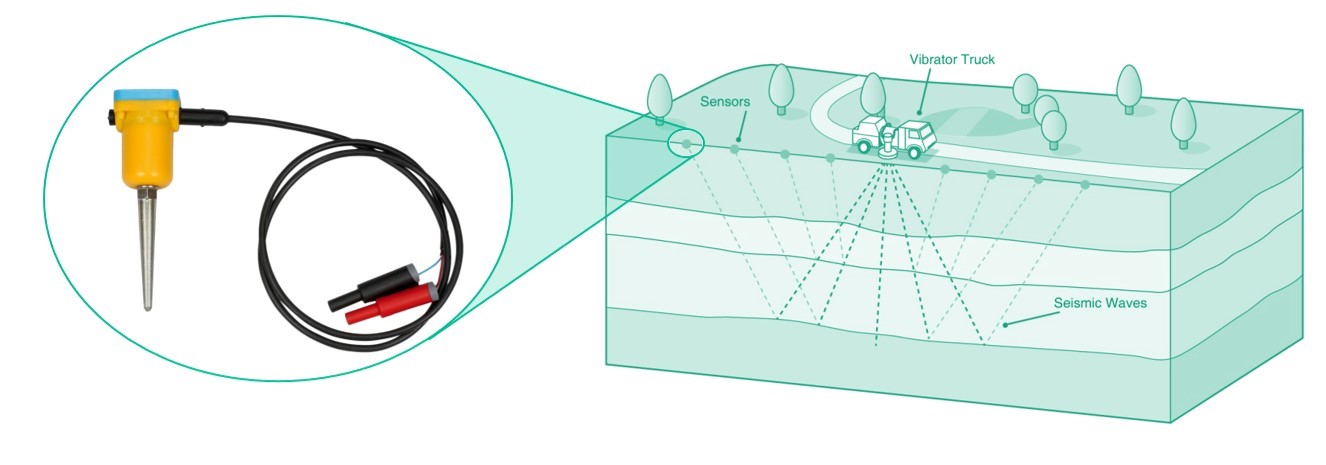
The primary application for moving-coil velocity sensors is very low frequency applications where the physics dictate that velocity levels will be much larger than the corresponding acceleration levels, and the acceleration signal itself will be miniscule. Rather than resorting to elaborate signal processing that attempts to extract meaningful information from something buried in the noise floor of the sensor, it is prudent to simply select a better transducer for the task. A notable machinery examples is hydroelectric turbines where casing vibration is measured but no higher frequencies (such as from rolling element bearings) are required. A notable non-machinery example is in petroleum exploration where vibrator vehicles shake the ground at very low frequencies and then measure the reflected seismic signals to detect the presence of underground petroleum deposits (Figure 5). Moving-coil devices (called geophones) are the sensor used to measure the reflected seismic vibrations.
Comparison
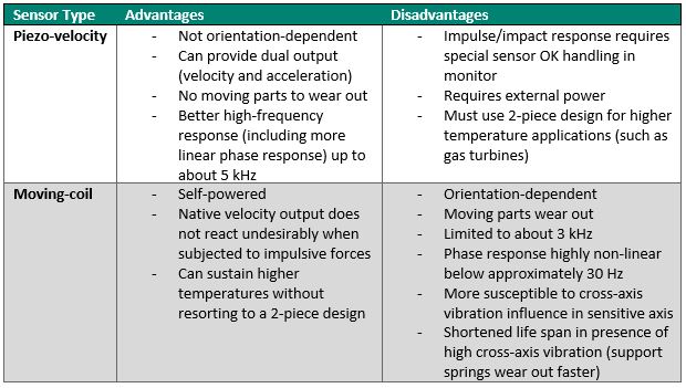
The table below compares salient aspects of piezo-velocity and moving-coil technologies.
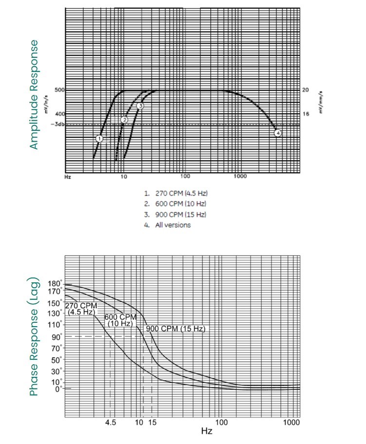
Phase Shift
The remark in the comparison table about phase response merits further examination. Consider the amplitude (top) and phase (bottom) response for a typical Bently Nevada moving-coil velocity sensor (model 9200) shown in Figure 6. It is immediately apparent that although the amplitude response is quite linear out to about 1000 Hz and does not drop off to the -3dB point until about 3500 Hz, the phase response is highly non-linear below approximately 30 Hz. This has to do with the resonant frequency of the spring support mechanism in the sensor. Although the amplitude response can be linearized, the phase response cannot. This becomes important in machinery diagnostic applications where phase is used and also in machinery balancing applications where the machine runs at speeds below 30 Hz (1800 rpm). In contrast, the mounted resonance of a typical piezo-velocity sensor such as the Bently Nevada 330500 is about 12 kHz and thus exhibits highly linear amplitude and phase response over the entire intended range of the sensor (4.5 Hz – 5 kHz).
Summary
We hope this examination of moving-coil versus piezo-velocity technology has helped you to understand the advantages, disadvantages, and suitable applications for each technology. Although for most intents and purposes, an integrating accelerometer such as the Bently Nevada Velomitor® sensor can be treated as having a native velocity output, there are some instances in which the integrated nature of the signal becomes apparent; notably, when impact/impulse forces act on the sensor. Bently Nevada’s recommended applications for these sensors account for these issues, including on reciprocating compressors. In most cases, a piezo-velocity sensor is the right choice and a moving-coil sensor introduces more disadvantages than advantages.
We will wrap up this series on accelerometers in the December 2021 issue of Orbit with Part 3: MEMS accelerometers. Although MEMS technology has been available for more than a decade, it has only recently progressed to the place where it can play a valuable role in machinery condition monitoring applications.

Chris McMillen
Senior Product Manager
BIO
Chris is the Senior Product Line Manager for Bently Nevada sensors. He is responsible for new developments and lifecycle management within the Bently Nevada sensor portfolio for both wired and wireless solutions.