

What are the characteristics of sound beams in ultrasonic testing?
In this article:
- Ultrasonic Sound Beams Exhibit Strong Directionality: Due to high-frequency oscillations and short wavelengths, ultrasonic waves propagate in narrow, concentrated beams where significant sound pressure is confined to a defined region known as the sound beam.
- Near and Far Fields Define Sound Pressure Behavior: The near field—located directly in front of the transducer—is marked by complex interference patterns, while the far field exhibits a predictable pressure decay, allowing for consistent measurements at greater distances.
- Beam Divergence and Width Are Mathematically Predictable: The divergence of a sound beam and its usable width are defined by equations involving frequency, wavelength, and transducer geometry, critical for targeting flaws precisely during inspections.
- Directional Sensitivity Determines Probe Effectiveness: The probe’s working range depends on how well it can transmit and receive sound from off-axis locations, quantified by directional factors and corresponding amplitude reductions.
- Sound Beam Characteristics Guide Accurate Inspections: Understanding beam width, divergence angles, and near-field length is essential for selecting the right probe, positioning it effectively, and interpreting ultrasonic signals with high accuracy.
- Waygate Technologies Enables Precision Through Advanced Beam Modeling: Waygate’s Krautkrämer phased array and conventional UT systems incorporate sophisticated software that visualizes beam geometry, models sound field behavior, and optimizes inspection setups—ensuring that users fully leverage beam characteristics for accurate, code-compliant results.
Due to the high number of oscillations (MHz) in an ultrasonic wave and the correspondingly small wavelength the sources of ultrasound have a strong directional characteristic. Sound pressure amplitudes p worth mentioning can only be confirmed in a small sector of space.
The essential and, for the test, the most significant portion of the sound field lies within a narrow sector of the field and this sector is known as the sound beam.
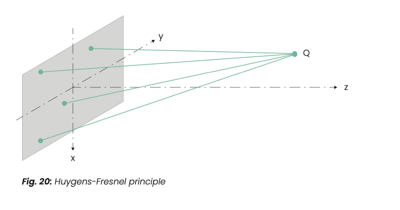
To understand this directional effect the surface of the transducer is regarded es being an array of sound radiating points. Each sound wave radiated from such a point propagates spherically. They reach a point Q in space at different transit times (fig. 20). There the separate waves overlap, they interfere and, according to phase and amplitude, give the total sound pressure at point Q.
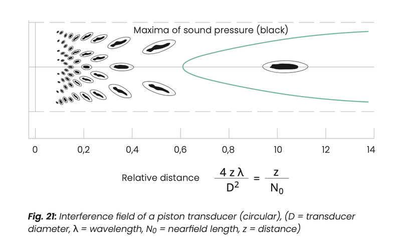
Depending upon the position of Q the effects of the interference can be very different. Fig. 21 shows how the sound is bundled into a narrow sector, due to interference, with a crystal where D/λ = 10. In the zone immediately in front of the transducer there is an area with strong sound pressure variations i. e. the “near field”.
The pressure maximum which is furthest away from the transducer marks the end of the near field. At this point the sound beam is concentrated to the greatest extent. Each source of sound has such a near field the shape of which, however, is influenced by the shape and size of the transducer.
Working Range and Directional Factor of the Probe
When testing materials, it is very important to know which portion of the sound beam is suitable for the testi.e. the working range of the probe. Frequently the question is posed: Where with a discshaped flat transducer, are the edges of the beam in which an echo from a point reflector does not decrease by more than a definite value below the maximum pressure on the axis. If a probe has a directional factor R = 1 on the acoustical axis then it generates, in a point Q outside the axis, a pressure R < 1.
A sound wave reflected from there is picked up by the same probe with the same reduced value R < 1. The returning signal, independent from the reflector (point) is located with the directional factor R2 as compared to the acoustical axis. In the dB system:
(9) 20 lg (R2) = 2 ∙ 20 lg (R)
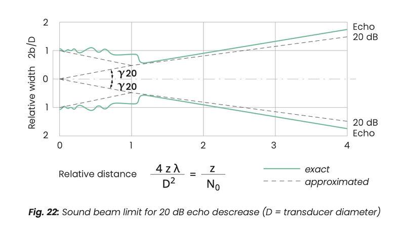
A 20-dB amplitude drop from a point reflector echo means then a free field decrease by 20/2 dB = 10 dB. Fig. 22 shows this beam limitation in the far field accurately and in the near field as enveloping. There isn't any sound pressure worth mentioning outside this beam. Fig. 22 then is the model for the sound radiation of a probe.
The near field shows a beam with the approximate diameter of the crystal—it is reduced however up to the end of the near field to half the crystal diameter.
Sound Beam Divergence
The divergence angle γ is constant because the sound pressure amplitude p normal to the acoustical axis for the disc-shaped crystal follows the following equation (10):
(10) p = 2 J1 (πλ Dsin𝛄) 0 (πλ Dsin𝛄)
(Besselfunktion J1(x))
For rectangular crystals the follow- ing applies accordingly:
(11) p = sin (πλ ssin𝛄) 0 (πλ ssin𝛄)
Whereby for s one uses either side a or b of the crystal.
Fig. 23 shows the sound pressure cross-distribution in the far field.
As per equations 10 and 11 and fig. 23 the following angles of divergence 𝛄6 and 𝛄20 also belong to the important cases of drops in amplitude by 6 dB and 20 dB:
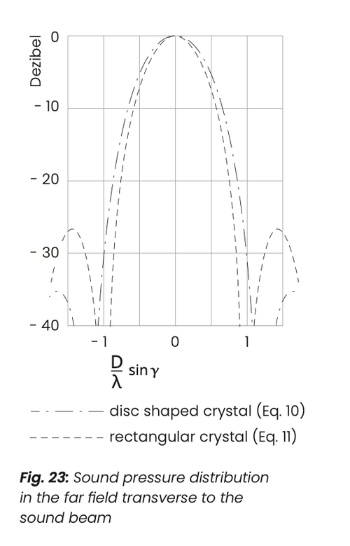
For disc oscillators:
𝛄6 = arc sin (0,51 λ/D) 𝛄20 = arc sin (0,87 λ/D)
for rectangular oscillators:
𝛄6 = arc sin (0,44 λ/s) 𝛄20 = arc sin (0,74 λ/s)
(s = an optional side a or b of the oscillator.)
Sound Pressure Variation with Distance
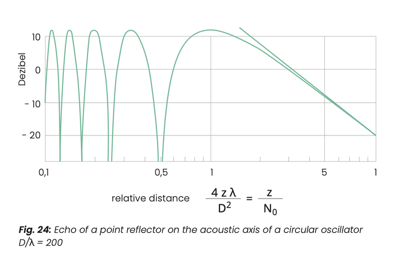
With distance z from the transducer the sound pressure p changes as well. The following applies for a disc- shaped transducer (12):
(12) p(z)=sinπ(D+z2-z p0 λ4
(Figure 24) D = transducer diameter, z = distance
For larger distances z equation (12) can be approximated by (13):
(13) p(z)≈πD2∙1 p0 4λz
in the dB system this becomes:
(14) 20lg(p(z)/p0)=20lg(πD /4𝛄)
-20lgz=const. -20lgz
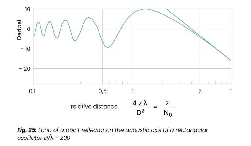
The following applies to all transducers regardless of their shape: For large distances the sound pressure amplitude decreases in proportion to the distance (equation 13) or:
the sound pressure curve plotted against the logarithm of the distance (equation 14) is a straight line. The area to which this relationship applies is known as the “far field”.
The range between the near field and the far field is known as the “transition range”. The distance law for a square transducer, which can't be described as easily as in equation 12 is given in fig. 25.
Beam Width and Near Field Length
The beam width (measured against the axis) is then calculated as:
λ (15)b≈z∙D
(for -6 dB amplitude drop to the acoustic axis)
The nearfield length N0 is calculated by:
(16) N0= D2 = D2∙f 4λ 4c
D = crystal diameter [mm] λ = wave length [mm]
c = sound velocity [km/s]
f = frequency [MHz]
In summary
In conclusion, the characteristics of sound beams in ultrasonic testing are governed by fundamental physical principles, notably interference and diffraction. The distinct regions of the sound field – the near field, transition range, and far field – each exhibit unique properties regarding sound pressure distribution and beam divergence.
Understanding these characteristics, including directional factors, amplitude drop-offs, and near field length, is critical for optimizing probe selection and interpreting test results accurately. The mathematical models and empirical observations presented herein provide a robust framework for predicting and managing sound beam behaviour, thereby ensuring the efficacy and precision of ultrasonic material inspections.
Further information on the near and far field can be found in the follow- ing publications:
[2] J. & H. Krautkrämer: Ultrasonic testing of materials, Springer- Verlag, Berlin (1990)
[8] U. Schlengermann: Über die Ver- wendung der Begriffe Nahfeld und Fernfeld in der Ultraschall-Werkstoff- prüfung (On the use of the terms near field and far field in the ultra- sonic testing of materials), Materi- alprüfung 15 (1973) no 5, 161—166