

What are the characteristics of sound fields in ultrasonic testing?
In ultrasonic testing of materials, understanding the behaviour of sound is fundamental. Unlike a confined beam of light, sound, by its very nature, creates a field that extends throughout space. This concept of a sound field is central to how ultrasonic pulses interact with and reveal discontinuities within a material.
By definition a sound field has no boundaries. A sound pressure amplitude can be correlated to every point in space (could be zero). The set of such position and sound pressure values forms the sound field, or more precisely the field of alternating sound pressure.
Static vs. Dynamic Sound Fields
The ultrasonic pulse technique functions, as the name implies with ultrasound pulses. These pulses need a certain time, depending upon the sound velocity c and the position of the sound source to form the maximum sound pressure at a specific location.
As the sound pressure builds up and decays at the pulse repetition frequency of up to 10,000 times per second one can neglect the time dependency and regard the sound field as if the pressure was constant at each point and equal to the maximum sound pressure there. The dynamic sequence of transmitting and receiving pulses leads to a practically static sound pressure field.
Probe-Generated Sound Fields and Discontinuity Detection
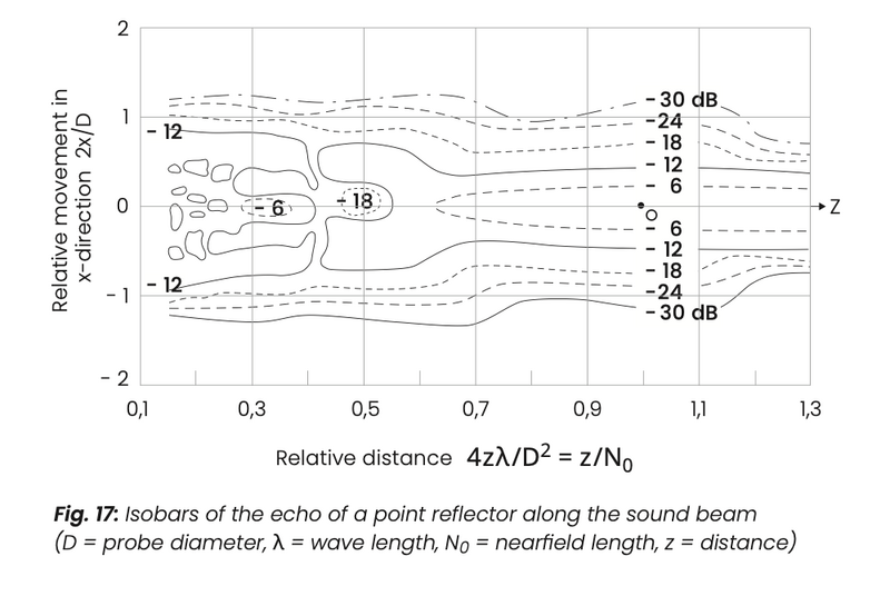
Each sound source has its characteristic type of pressure distribution in space and it isn't the probe but rather this sound field generated by it which is a means by which discontinuities are detected in the material being tested, fig. 17.
Representing Sound Fields: Isobars and Directional Characteristics
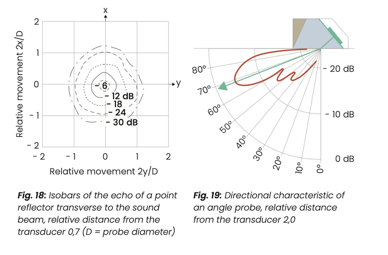
To show a field of sound pressure by means of a diagram one usually marks those lines in a cross section in space where there is a constant sound pressure (isobars) (fig. 17, 18). The -6 dB curve means that on this line the pressure is 6 dB below the pressure at the 0 dB position i. e. it is only half as big as at the 0 dB position.
Contrary to the isobar representation (fig. 17, 18) where for every sound pressure p the location is also given where it is present, the directional characteristic (fig. 19) which is to be measured at a certain distance from the sound source gives only the di- rection in which this pressure can be measured. The directional characteristic thus can only apply for the distance in which it has been taken.
Free Fields vs. Echo Fields
The description of a sound field given here is based on the fact that, using a suitable point receiver, the sound pressure in every point in space is measured without interfering with the sound field. Thus, it is known as the free field, i. e. a free radiation of the sound source or the free field directional characteristic.
If, however, the sound wave is reflected at a reflector in a certain field point and is received by the same probe one obtains the echo field characteristic in reference to the reflector used. For the pulse- echo-method the free field data is less interesting than the echo fields which however do not only depend upon the probe but depend just as much on the reflector used.
In summary
The concept of a sound field is central to the efficacy of ultrasonic material testing. While initially appearing complex due to its time-varying nature, the effective static sound pressure field provides a consistent basis for analysis.
The unique pressure distribution characteristic of each sound source, rather than the probe itself, is the primary means by which material discontinuities are identified. Visualizations such as isobars and directional characteristics provide crucial insights into these fields, though it is the echo field—reflecting the interaction with specific reflectors—that holds paramount interest for the pulse-echo method employed in practical testing. A thorough understanding of these sound field properties is therefore essential for accurate and reliable material evaluation.
Information about sound fields and sound field data give:
[2] J. & H. Krautkrämer: Ultrasonic testing of materials, Springer- Verlag, Berlin (1990)
[3] W. Lehfeldt: Ultraschall kurz und bündig (Ultrasonics—short and concise) Vogel-Verlag, Würzburg (1973)